Bayesian Updating for Log Returns

A Practical Approach

In this post, we'll explore how Bayesian updating can be applied to log returns of a financial asset. We'll adapt the concepts from the articles "Bayesian Coin Flips" by Thomas J. Fan and the Code Chalet to work with log returns instead of coin flips.

Introduction

Imagine you're analyzing the log returns of a stock. Log returns are the natural logarithm of the ratio of consecutive prices of a financial asset, commonly used due to their additive properties and the assumption of normality over long periods. You want to update your belief about the average log return of this stock as new data comes in, using Bayesian methods.

We'll walk through a Bayesian analysis of log returns, starting with prior beliefs, updating them with observed data, and interpreting the results.

Data and Model

We model log returns as a random experiment with a continuous outcome. The log returns follow a normal distribution with an unknown mean (μ) and a known variance (σ²). Our goal is to update our belief about the mean log return using observed data.

Prior Distribution

We start with a prior distribution representing our initial belief about the mean log return. Suppose we have no strong reason to believe the stock has a high or low return; we can use a normal prior distribution with mean 0 and a large variance.

\(\text{Prior: } \mu \sim N(\mu_0, \tau_0^2)\)

For our example:

\(\begin{align*} & \bullet \ \mu_0 = 0 \\ & \bullet \ \tau_0^2 = 0.01^2 \end{align*} \)

This is equivalent to having a uniform prior belief over a range of possible means for the log return.

Let's visualize this prior:

import numpy as np
import matplotlib.pyplot as plt
from scipy.stats import norm

# Define the prior distribution
mu_0 = 0
tau_0 = 0.01
x = np.linspace(-0.05, 0.05, 1000)
prior = norm.pdf(x, mu_0, tau_0)

# Plot the prior distribution
plt.figure(figsize=(10, 6))
plt.plot(x, prior, label='Prior Distribution')
plt.title('Prior Distribution of Mean Log Return')
plt.xlabel('Mean Log Return')
plt.ylabel('Density')
plt.legend()
plt.show()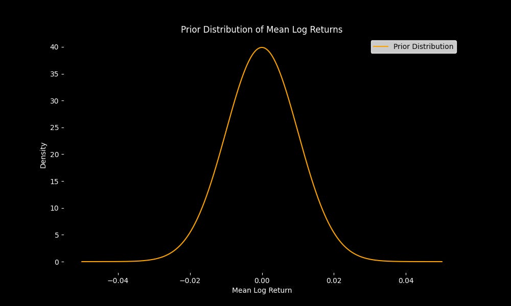

---

Likelihood

Next, we observe log returns and use this data to update our prior. Suppose we observe the following log returns:

\(x_1, x_2, \ldots, x_n \)

The likelihood is the probability of observing this data given a certain mean log return. Since we assume log returns follow a normal distribution, the likelihood is also normal:

\(\text{Likelihood: } x_i \sim N(\mu, \sigma^2)\)

Posterior Distribution

Using Bayesian updating, we combine our prior and likelihood to obtain the posterior distribution. The posterior distribution is also normal, with updated parameters:

\(\begin{align*} \mu_n &= \frac{\tau_0^2 \sum_{i=1}^n x_i + \sigma^2 \mu_0}{n \tau_0^2 + \sigma^2} \\ \tau_n^2 &= \frac{\sigma^2 \tau_0^2}{n \tau_0^2 + \sigma^2} \end{align*}\)

Python Implementation

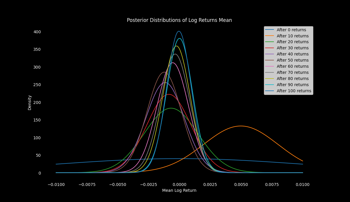
Let's implement this in Python and visualize the updating process

import numpy as np
import matplotlib.pyplot as plt
from scipy.stats import norm

# Generate synthetic log returns
np.random.seed(42)
n_returns = 100
true_mean = 0.001  # True mean of log returns
true_variance = 0.0001  # True variance of log returns
log_returns = np.random.normal(true_mean, np.sqrt(true_variance), n_returns)

# Initial prior parameters
mu_prior = 0  # Prior mean
tau_prior = 0.01  # Prior standard deviation
sigma = np.sqrt(true_variance)  # Known standard deviation of log returns

# Lists to store the posterior parameters after each log return
mu_posteriors = [mu_prior]
tau_posteriors = [tau_prior]

# Perform Bayesian updating for each log return
for log_return in log_returns:
    # Update the posterior mean and variance
    tau_posterior = np.sqrt(1 / (1 / tau_prior**2 + 1 / sigma**2))
    mu_posterior = tau_posterior**2 * (mu_prior / tau_prior**2 + log_return / sigma**2)
    
    # Store the updated parameters
    mu_posteriors.append(mu_posterior)
    tau_posteriors.append(tau_posterior)
    
    # Update prior for next iteration
    mu_prior = mu_posterior
    tau_prior = tau_posterior

# Plot the posterior distributions
x = np.linspace(-0.01, 0.01, 1000)

plt.figure(figsize=(12, 8), facecolor='black')
ax = plt.gca()
ax.set_facecolor('black')

for i in range(0, n_returns + 1, 10):
    plt.plot(x, norm.pdf(x, mu_posteriors[i], tau_posteriors[i]), label=f'After {i} returns')

plt.title('Posterior Distributions of Log Return Mean', color='white')
plt.xlabel('Mean Log Return', color='white')
plt.ylabel('Density', color='white')
plt.legend()
plt.xticks(color='white')
plt.yticks(color='white')
plt.show()

Interpreting the Model

The posterior distribution gives us updated beliefs about the mean log return after observing the data. If we were to predict the next period's log return, we could use the posterior mean as our best estimate.

Mathematical Formulas

Let's delve into the mathematical details:

• Posterior Mean:

\(\mu_n = \frac{\tau_0^2 \sum_{i=1}^n x_i + \sigma^2 \mu_0}{n \tau_0^2 + \sigma^2} \)

where:

\(\begin{align*} & \bullet \ \mu_0 \text{ is the prior mean.} \\ & \bullet \ \tau_0^2 \text{ is the prior variance.} \\ & \bullet \ x_i \text{ is the i-th observed log return.}\\ & \bullet \ \sigma^2 \text{ is the known variance of log returns.} \end{align*}\)

• Posterior Variance:

  \(\tau_n^2 = \frac{\sigma^2 \tau_0^2}{n \tau_0^2 + \sigma^2}\)

• These formulas allow us to iteratively update our beliefs about the mean log return as new data arrives.

  Conclusion

  This approach demonstrates how Bayesian updating can be applied to log returns, providing a dynamic way to refine our estimates of the mean log return as new data arrives.
  

  By following these steps, we can continuously update our model with new data, allowing for more accurate predictions and better decision-making in the financial markets. The Python implementation provided offers a practical way to visualize and apply these concepts in a real-world context.